cProfile

cProfile is a function-level profiler that is part of Python’s standard library. It is a command-line profiler, that can also be called directly from Python. 3rd party packages such as snakeviz can be used to visualise it’s output in a web browser or Jupyter Notebook.

QuickStart

It can be called directly within your Python code as an imported package, however it’s easier to use it’s script interface:

python -m cProfile <script name> <arguments> > <output file>

For example if you normally run your program as:

python my_script.py input.csv

You would call cProfile to produce profiling output analysis.txt with:

python -m cProfile my_script.py input.csv > analysis.txt

No additional changes to your Python code are required, it’s really that simple!

Interpreting Output

The output file analysis.txt can be opened with a text editor, it contains a table that identifies functions in order of the proportion of execution time they occupied.

         28 function calls in 4.754 seconds

   Ordered by: standard name

   ncalls  tottime  percall  cumtime  percall filename:lineno(function)
        1    0.000    0.000    4.754    4.754 my_script.py:1(<module>)
        1    0.000    0.000    1.001    1.001 my_script.py:13(b_2)
        3    0.000    0.000    1.513    0.504 my_script.py:16(c_1)
        3    0.000    0.000    1.238    0.413 my_script.py:19(c_2)
        3    0.000    0.000    0.334    0.111 my_script.py:23(d_1)
        1    0.000    0.000    4.754    4.754 my_script.py:3(a_1)
        3    0.000    0.000    2.751    0.917 my_script.py:9(b_1)
        1    0.000    0.000    4.754    4.754 {built-in method builtins.exec}
       11    4.753    0.432    4.753    0.432 {built-in method time.sleep}
        1    0.000    0.000    0.000    0.000 {method 'disable' of '_lsprof.Profiler' objects}

The columns have the following definitions:

Column	Definition
ncalls	The number of times the given function was called.
tottime	The total time spent in the given function, excluding child function calls.
percall	The average tottime per function call (tottime/ncalls).
cumtime	The total time spent in the given function, including child function calls.
percall	The average cumtime per function call (cumtime/ncalls).
filename:lineno(function)	The location of the given function’s definition and it’s name.

Visualising Output

For more complex programs the former output will grow and can become harder to interpret. Instead, an output file -o <output_file> can be passed to cProfile which can be interpreted by 3rd party packages such as snakeviz to provide an interactive visualisation.

First it’s necessary to install snakeviz, it should be available via pip.

pip install snakeviz

Then cProfile can be executed, specifying an output file with -o

python -m cProfile -o <output file> <script name> <arguments>

For example if you normally run your program as:

python my_script.py input.csv

You would call cProfile to produce profiling output out.prof with:

python -m cProfile -o out.prof my_script.py input.csv

Then out.prof is passed to snakeviz:

python -m snakeviz out.prof

This should open snakeviz’s visualisation of the profiling results in your web browser

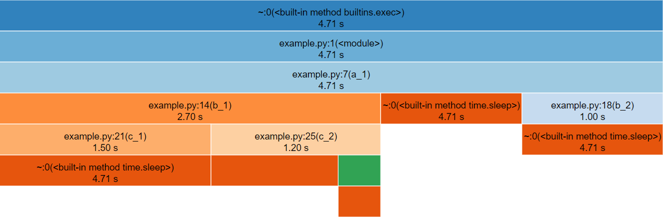
Figure 1: An example of the default ‘icicle’ visualisation provided by snakeviz.

The icicle diagram displayed by snakeviz represents an aggregate of the call stack during the execution of the profiled code. The box which fills the top row represents the the root call, filling the row shows that it occupied 100% of the runtime. The second row holds the child methods called from the root, with their widths relative to the proportion of runtime they occupied. This continues with each subsequent row, however where a method only occupies 50% of the runtime, it’s children can only occupy a maximum of that runtime hence the appearance of “icicles” as each row gets narrower when the overhead of methods with no further children is accounted for.

By clicking a box within the diagram, it will “zoom” making the selected box the root allowing more detail to be explored. The diagram is limited to 10 rows by default (“Depth”) and methods with a relatively small proportion of the runtime are hidden (“Cutoff”).

As you hover each box, information to the left of the diagram updates specifying the location of the method and for how long it ran.

Jupyter Notebooks

If you’re more familiar with writing Python inside Jupyter notebooks you can still use snakeviz directly from inside notebooks using the notebooks “magic” prefix (%) and it will automatically call cProfile for you.

First snakeviz must be installed and it’s extension loaded.

!pip install snakeviz
%load_ext snakeviz

Following this, you can either call %snakeviz to profile a function defined earlier in the notebook.

%snakeviz my_function()

Or, you can create a %%snakeviz cell, to profile the python executed within it.

%%snakeviz

def my_function():
    print("Hello World!")

my_function()

In both cases, the full snakeviz profile visualisation will appear as an output within the notebook!

You may wish to right click the top of the output, and select “Disable Scrolling for Outputs” to expand it’s box if it begins too small.

Limitations

cProfile is a deterministic profiler, rather than a sampling profiler, this means that it captures all function calls. This causes the profiler to have a high profiling overhead, which may lead to the profiling execution being significantly slower for code that includes many function calls.