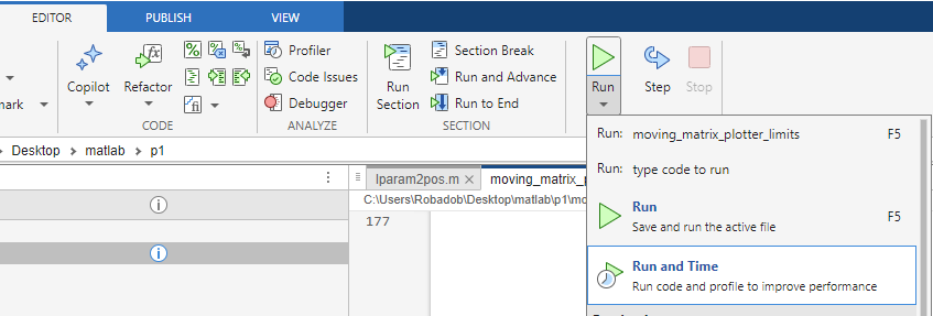
Run and Time
The MATLAB desktop application (as opposed to the MATLAB web application) has built in profiling tools, which can be used to easily provide a visual insight to where time is being spent during your code’s execution. This doesn’t necessarily require any changes to your code, merely executing it with the button labelled “Run and Time”.
QuickStart
- Open your code with the MATLAB Editor, as you would normally would when working on it.
- Click “Run and Time”, which can be found in the drop-down menu of the regular “Run” button (see Figure 1 (above)).
- After your code exits successfully, a new window “Profiler” will open containing your profiling results.
Reducing Profile Scope
Profiling captures extra information during your code’s execution, this both slows down the execution and may produce a large amount of data.
By default, MATLAB has a profiler history size of 5 million function calls to limit the size of the data collected. If this value is exceeded, some profiler features (such as the Flame Graph) will not be available.
To make profiling as useful as possible, it’s recommended where feasible to profile a small but representative example so that it executes in 1-2 minutes. This could be as simple as reducing the number of iterations, or the problem size.
If your code is too complicated, or scales such that this approach is impractical. You can instead enable and disable the profiler dynamically during execution to profile a particular part of your code using the command profile and then execute it normally.
% MATLAB code
% ...

% Enable the profiler
profile on

% MATLAB code to be profiled
% ...

% Disable the profiler
profile off

% More MATLAB code
% ...

% Open the profile report (if not already open)
profile viewer
You should only enable and disable the profiler once during execution, as each time it is re-enabled the data that was previously collected will be discarded.
Ensure that you remove or comment these lines once you’ve finished profiling, as executing your code with the profiler enabled will reduce your code’s performance.
Interpreting Output
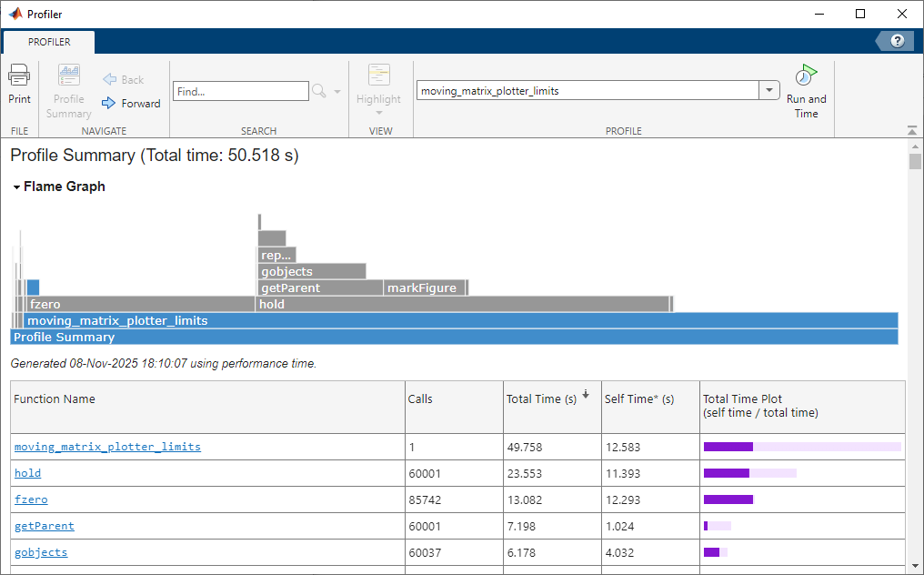
The initial page displayed within the profiler window is the Profile Summary, which presents a Flame Graph and a table listing the functions called alongside their execution time. This page can be returned to at any time, by clicking the “Profile Summary” button in the top-left corner of the profiler.
Flame Graph
If the flame graph section states “Flame graph is not available…”, try reducing the scope of the profile as too much data was collected. If you can’t see that message or the graph, make sure the flame graph accordion is expanded.
Flame graphs are a common approach to visualising aggregate function-level profiling data (or if vertically reflected, called an icicle graph). The bottom row of the flame graph is the root of the profile which occupies 100% of the runtime, this is shown to be the “Profile Summary”. Each row above this shows the most expensive functions (or files) executed by the previous row, producing a hierarchical visualisation of where time was being spent during execution. Each function will only appear as a child of the function it was called within once, as multiple child-calls to the same function are aggregated. As rows progress up the graph the proportion of the graph’s width occupied by cells typically reduces, producing the flame (or icicle) pattern the graph is named after. These gaps represent the execution time of the function that was not spent executing child functions, e.g., basic arithmetic and control flow.
If a particular cell of MATLAB’s flame graph is hovered with the mouse cursor, a tool tip appears saying the percentage runtime (equivalent to the cell’s width) and absolute runtime of that function including child function calls. Grey cells represent MATLAB functions, and blue cells represent your code.
In Figure 2 (above) it’s clear that moving_matrix_plotter_limits was the most expensive function (98.5% of the runtime), that’s because we profiled moving_matrix_plotter_limits.m. The row above show that fzero and hold within moving_matrix_plotter_limits.m occupied 25.9% and 46.6% of the runtime respectively. That would suggest that those functions, and how are they are being used, should be investigated.
If a cell within the flame graph is clicked, it will navigate to a profile summary for the selected cell’s file or function.
Profile Summary Table
The table beneath the flame graph lists each of the functions called in order of their total execution time. This provides the same information as the flame graph, however it includes all functions called including very quick ones which would be difficult to visualise in the flame graph.
The table has 5 columns:
- Function Name, The name of the relevant function or file.
- Calls, The number of times that function (or file) was called.
- Total Time, The absolute time spent executing that function, including child function calls.
- Self Time, The absolute time spent executing that function, excluding child function calls.
- Total Time Plot, A bar representing the total time and self time, with respect to the total runtime of the profile. This is how it would appear within the flame graph as a child of the root.
If a function name is clicked within the table, the profiler will navigate to a profile summary for the selected function which contains both function-level and line-level information.
File/Function Profile Summary
These profile summaries are available for core MATLAB functions, however it’s normally best to focus on your own files and functions.
The function profile summary contains several sections:
Flame Graph
A flame graph scoped such that the selected function occupies the full width. This can surface greater child calls which weren’t visible in the profile summary’s flame graph.
Parents
A table of parent functions which called this function and how many times they were called. This data is aggregated, so it won’t uniquely identify individual locations if a function was called from multiple places within the same parent file or function. If there was no calling function, this section will state “No parent”.
Lines that take the most time
A table listing the most expensive lines of code.
The table has 6 columns:
- Line Number, The line number of the specific line of code within the affected file.
- Code, The particular line of code.
- Calls, The number of times that line of code was executed.
- Total Time, The absolute time spent executing that line of code.
- % Time, The total time spent executing that line, relative to the time spent executing the parent function.
- Time Plot, A bar representing the total time, with respect to the total time spent in the current file or function.
Clicking a line number in the table, will jump down to that specific line in the Function Listing section below.
Children
A table of child function calls, and their respective execution times. This is similar to the profile summary page’s table, however the “Self Time” column has been replaced with “% Time” which represents the total time relative the parent function’s execution time. If no child functions were called, this section will state “No children”.
Code Analyzer results
The code analyzer performs static analysis of your code to provide a list tips for how you can improve specific lines of your code. Most of these tips won’t be relevant to your code’s performance, but they may help you to avoid bugs and make your code easier for others to parse.
Function listing
This final section of the function profile report, presents the source of the selected file or function preceded by 3 columns which list:
- Time, The absolute time spent executing that line of code.
- Calls, The number of times that line of code was executed.
- Line, The number of that line of code within the relevant file.
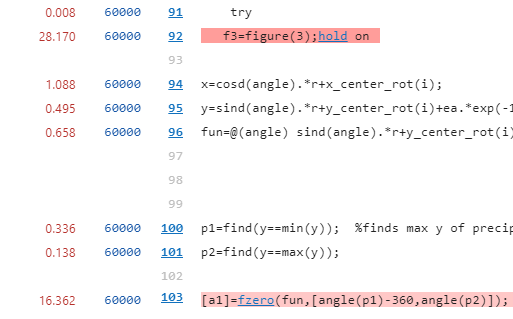
The most computationally expensive lines of code within the listing will have a red background. The darkness of the red background represents how expensive the line of code is, with more expensive lines having darker backgrounds. This visual cue allows the hot-path to be quickly identified.
Limitations
MATLAB’s inbuilt profiler is intuitive and thorough, the only likely difficulties you may run into would be if you are profiling complex code which uses parallelisation (e.g. parfor) or GPU computation. If you do come across this challenge, try adjusting your code so that you can profile a serial version. Any significant serial optimisation will translate to a parallel speed-ups, so don’t feel the need to struggle with parallel profiling.
If you’re keen to attempt profiling your GPU code, MATLAB provides the separate GPU performance analyzer.