Getting Started
This article is approximately 4000 words, and is expected to take 20 minutes to read.
If you’re new to learning about performance (and using this website), this long-form introduction is a great place to start. The Reasonable Performance Computing SIG website is intended to provide enough introductory software performance material to get beginners started identifying and (hopefully) resolving performance traps in their own code.
If you’re already familiar with the basics, perhaps you want to skip ahead.
- Introduction to Profiling
- Profiling Tools
- How to Profile
- Interpreting Results
- Identifying Optimisations
- Case Studies
- Key Points
Introduction to Profiling
Profiling is the practice of executing code whilst collecting granular metrics, in particular performance profilers collect information to help reveal where time is being spent in the code during execution. The information collected ranges from the time spent executing each function or line of code, to low-level hardware metrics such as achieved memory bandwidth. Profiler output narrows the scope for optimisation from the entire codebase to potentially just a handful of lines, enabling quick identification of issues that might otherwise be overlooked.
Regardless of experience, whether a self-taught or trained programmer, it’s always possible to introduce small inefficiencies into your code that significantly impact performance. These may not impact the correctness of your results, so it’s easy for them to go overlooked. Perhaps you added some crude validation code whilst debugging, then months later you’ve scaled up several orders of magnitude and forgotten about the validation code (as the same bug hasn’t resurfaced) but it’s now accounting for a significant proportion of your code’s runtime. Or maybe you’re simply unfamiliar with a performant feature of a library or language that you’ve used.
Profiling tools are designed to uncover where time is being spent executing your code, helping to reduce the volume of code worth investigating for performance optimisations. As Donald Knuth famously observed, we should only focus our attention on optimising the critical 3% of our code:
Programmers waste enormous amounts of time thinking about, or worrying about, the speed of noncritical parts of their programs, and these attempts at efficiency actually have a strong negative impact when debugging and maintenance are considered. We should forget about small efficiencies, say about 97% of the time: premature optimization is the root of all evil. Yet we should not pass up our opportunities in that critical 3%.
To quantify this idea, we can use Amdahl’s law which shows that the overall performance improvement from optimising a single part of a system is limited by the fraction of time that the improved part is actually used. Figure 1 provides an interactive graph where you can explore changing the proportion of runtime optimised (P).
For example, if a function which accounts for 20% (P=0.20) of the total application runtime was improved to be 128x faster then the total performance improvement would be less than 1.25x. This shows why we should focus optimisation attention on the significant components. There’s little value in making small optimisations to inexpensive sections of the runtime if it will have negligible impact to the overall performance.
However Amdahl’s law is theoretical. In practice, computer hardware is shared and bottlenecks may impact multiple components of the code. Hence, it’s possible for some optimisations to improve performance beyond the affected code. In one memorable example, profiling attributed slightly below 80% of the runtime to redundant object copies. Removing these led to a 10x speedup - even though Amdahl’s law would only predict a 5x speedup.
Profiling Tools
You may have previously tried to identify performance bottlenecks by manually timing sections of your code, for example by inserting timing calls around individual functions or blocks. While this can give you a rough idea of how long different parts of your code take to run, this approach is slow and unwieldy. It is difficult to achieve good coverage even for a moderately sized codebase, and the added instrumentation often requires ongoing effort to update, maintain, and eventually remove as a project evolves. Indeed, such efforts can ultimately contribute to performance degradation as they are forgotten.
In contrast, hot-path profiling (also known as hotspot profiling), requires little additional expertise if you understand your code, and can usually be integrated quickly into your workflow. It may immediately reveal an obvious bottleneck, confirm your assumptions about the most expensive parts of your code, or highlight areas that need further investigation. This is a low-cost exercise that either leads to tangible improvements or gives you greater confidence in the performance of your code.
Most programming languages have one or more tools for hot-path profiling. While these tools take different forms, the underlying concepts are highly transferable. Once you understand the core principles, you should be able to use them effectively across languages and frameworks.
Hot-path profiling typically operates at two levels, or a combination of both: function-level and line-level. Function-level profiling measures metrics for each function, including time spent both inclusive and exclusive of child function calls. Line-level profiling instead tracks execution time for each line of code. Although line-level profiling generates much more data, it can provide additional context when function-level metrics alone are insufficient.
For either level, hot-path profiling tools generally use one of two approaches to collect performance data. The simplest are deterministic profilers, which record every function call and every executed line of code. This method provides detailed insights, such as how many times each function is called or how often each branch of a conditional is executed. However, the high frequency of data collection carried out by deterministic profilers often has a significant computational overhead, increasing the time spent profiling and making them less desirable when profiling long workflows that would lead to collecting large amounts of data.
More advanced profilers typically use a sampling approach. In this method, the profiler periodically checks which line of code is executing, for example 1,000 times per second. The sample rate is usually configurable. Sampling captures only a fraction of the data collected by deterministic profilers, so it provides an approximate picture. However, this approximation is sufficient for our purposes. We are primarily interested in the most expensive parts of the code. If a function consumes a significant portion of runtime, for example 10% or more, it will normally appear proportionally in the samples. Sampling profilers therefore introduce much lower overhead, making them ideal for profiling long workflows.
It is not essential to memorise these differences. In most cases, you can simply use the profiler that is available. The key points are summarised in figure 2 below.
| Collection method | Attribution level | Strengths | Weaknesses |
|---|---|---|---|
| Sampling | Function | Minimal overhead | Statistical noise for small runs |
| Sampling | Line | Low overhead, fine-grained insight | Potentially biased by timing |
| Deterministic | Function | Exact call counts, timings | Moderate overhead |
| Deterministic | Line | Precise attribution, branching info | High overhead |
In addition to common hot-path profiling tools, you may come across more specialised profilers. In general these take two forms.
Firstly there are timeline profilers, these typically operate similar to function-level profilers however instead of presenting aggregations of the function-level metrics, they present function calls on a timeline of the code’s execution. Timeline profiling is particularly useful when investigating parallel codes as it clearly displays synchronisation points and idle threads. It may also be useful if profiling a code where performance degrades over runtime as this can be difficult to diagnose with aggregated metrics.
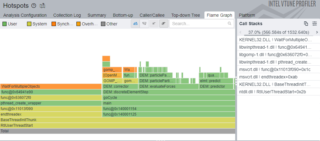
Secondly you may also come across “hardware metric” profilers. These are typically provided by hardware manufacturers (e.g. Intel VTune, AMD μProf & NVIDIA NSight Compute) and gather metrics from hardware-specific counters. They allow expert users to analyse data such as theoretical vs achieved memory bandwidth or floating-point operations per second. Interpreting these metrics correctly requires deeper knowledge, so it’s normal if they don’t immediately make sense. For most purposes, you can focus on hot-path profiling. Some of these tools, including Intel VTune, also offer a hot-path profiling mode, which needs to be selected when starting a profiling session.
In addition to performance profiling, profiling can sometimes refer to memory profiling. Memory profilers are designed for tracking memory allocations to help diagnose the source of memory leaks (when a program’s memory utilisation erroneously continues increasing) or merely high memory utilisation. While memory profilers are valuable for diagnosing memory issues, they are generally not helpful for evaluating overall software performance.
If your code is doing something more advanced such as distributed computing (e.g. MPI) or GPU compute (e.g. CUDA), the remaining guidance is unlikely to be of great help. You may find it useful to hot-path profile a serial version of the code, but in both these cases communication overhead can become the largest performance bottleneck which may not be well reflected in traditional profiling tools. Consider instead reaching out to HPC communities for support. Regional and national HPC centres often host events and training related to both writing and optimising distributed and GPU codes.
How to Profile
The best time to profile code is once development is complete and before it is put into use or published. As a codebase evolves, performance bottlenecks often shift. Code that accounts for a large fraction of runtime early on may become negligible later as features are added or implementations change.
During development, testing is frequently performed on small data sets or populations. Algorithms with poor scaling behaviour may therefore appear acceptable until they are executed at production scale, sometimes with data sets several orders of magnitude larger.
Although profiling unfinished code is not inherently wrong, it can be counterproductive. It risks diverting attention from core development, and optimising code that is still in flux can introduce subtle bugs that are hard to detect.
When your code is ready, decide what workflow you want to profile. The results are only meaningful for code paths that are actually executed, so the selected workflow should closely resemble the one you intend to optimise.
For highly configurable applications, it is usually best to choose a smaller or simplified configuration that is still representative of typical behaviour. This keeps profiling overhead manageable while still exercising the relevant performance-critical paths.
If the code is iterative, such as a simulation that runs for thousands of steps, profiling the full execution is often unnecessary. Since each iteration typically executes the same code, profiling only a subset of steps will usually produce similar insights at a much lower cost, aside from any one-time initialisation overhead. However, try to ensure the profiled steps are still representative of all major behaviours present in the full execution.
Be aware that profiling adds runtime overhead and will slow execution. To minimise time spent profiling, it is generally preferable to profile a configuration that runs for several minutes. If this is not feasible, profiling a longer or full configuration is still acceptable. In that case, note that some profilers stop collecting data once internal buffers are full, although if you run into this behaviour it can often be adjusted by configuring buffer sizes or delaying the point at which the profiler begins to collect data.
Most profilers can be used without modifying your project. The main exception is compiled languages such as C and C++, which typically require the build to be configured explicitly for profiling. This usually involves compiling with both debug symbols and compiler optimisations enabled. Debug symbols allow the profiler to map the compiled machine instructions back to locations in the source code, while compiler optimisations ensure that the profiled execution is representative of production.
Some profilers may also require limited changes to the code, such as explicitly marking functions to be profiled or controlling when data collection begins and ends. These requirements vary between tools and use-case, so you should consult the documentation for your chosen profiler to determine whether any configuration or code changes are necessary.
Interpreting Results
Once your code executes to completion via the profiler, you should be able to view the results. There are a few common approaches for how profilers present these results:
Flame and Icicle Graphs
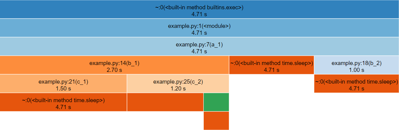
Flame graphs and icicle graphs are standard visualisations for aggregated, function-level profiling data. Flame graphs place the root row at the bottom and grow upwards, while icicle graphs place the root row at the top and grow downwards. Aside from orientation, they are interpreted in exactly the same way.
The root row always contains a single full-width cell, representing the entry point of the profiled execution, typically the main function. Above or below it, depending on the orientation, successive rows show cells corresponding to functions called by their parent. The width of each cell represents the aggregated runtime spent in that function, including time spent in its callees.
Child cells occupy some fraction of the width of their parent. Most functions spend time performing work other than calling child functions, such as control flow, arithmetic, or data manipulation. This unused space produces the stepped appearance characteristic of flame (Figure 3) and icicle (Figure 4) graphs, which gives them their names.
These graphs are typically interactive. Selecting a cell redraws the graph with that function as the new root, making it easier to inspect deeper call hierarchies that may otherwise be difficult to see.
Overall, flame and icicle graphs provide a concise visual overview of how execution time is distributed across function call hierarchies within a profiled program.
snakeviz.Table
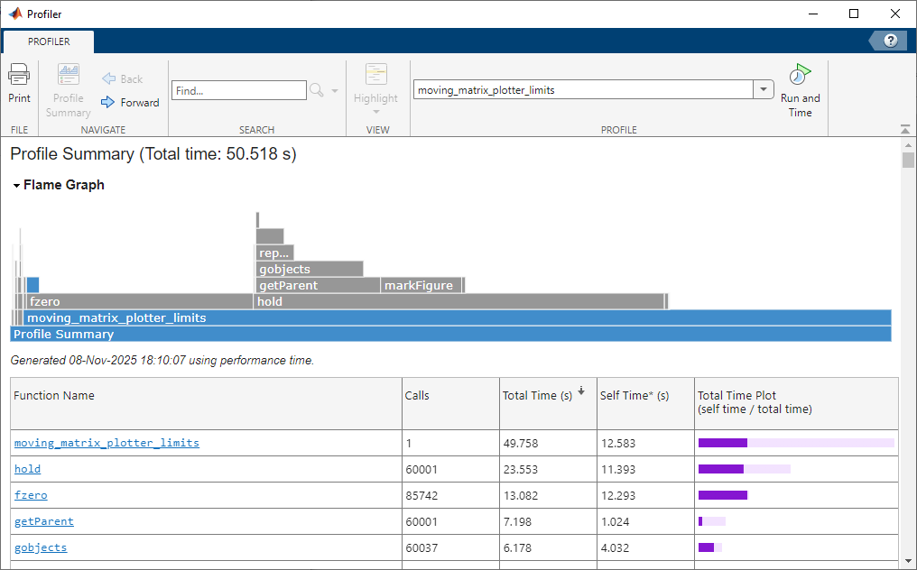
Another common way to present function-level profiling data is as a table, often referred to as a profile summary. This lists functions alongside their measured runtime, typically reported both inclusive and exclusive of time spent in child function calls. Some profilers also record how many times each function is invoked, allowing a per-call cost to be derived.
These tables provide a fast way to identify the most computationally expensive functions in a program. However, unlike flame or icicle graphs, they do not naturally convey call hierarchy or the context in which functions are executed.
Depending on the tool, the table may be interactive, allowing rows to be sorted or functions to be selected to jump directly to an annotated source code view (Figure 5). Other profilers provide only a static table representation (Figure 6).
Flat profile:

Each sample counts as 0.01 seconds.
  %   cumulative   self                self     total
 time   seconds   seconds    calls     s/call   s/call  name
 13.75     16.38    16.38 125676749836   0.00     0.00  tVect::operator+(tVect const&) const
 12.60     31.40    15.02  94039864750   0.00     0.00  tVect::operator*(double const&) const
 10.02     43.34    11.94     65081331   0.00     0.00  elmt::correct(double const*, double const*)
  8.54     53.52    10.18   4068178008   0.00     0.00  DEM::particleParticleCollision(particle const*...
  7.62     62.60     9.08   2392019595   0.00     0.00  elmt::predict(double const*, double const*)
  5.66     69.34     6.74  41323211762   0.00     0.00  tVect::operator-(tVect const&) const
  5.45     75.84     6.50  36306445222   0.00     0.00  quaternion::operator*(double const&) const
  4.74     81.49     5.65   7264658795   0.00     0.00  project(tVect, quaternion)
  4.60     86.97     5.48  32022205839   0.00     0.00  quaternion::operator+(quaternion const&) const
  3.61     91.27     4.30      2380119   0.00     0.00  DEM::evaluateForces()
  2.25     93.95     2.68  16726846623   0.00     0.00  tVect::cross(tVect const&) const
  ...
Inline Code
In contrast to function-level visualisations, line-level profiling results are typically presented inline with the source code. Each line is shown alongside profiling metrics in a pseudo-table layout (Figure 7), often using visual cues such as background shading to indicate relative cost (Figure 8). Lines with high execution time are commonly highlighted with colours, which get darker or warmer corresponding to each line’s expense, making hotspots immediately visible.
This inline representation provides a fast way to identify performance patterns within a function, particularly when scanning large files. It can reveal expensive loops, conditionals, or individual operations that are not obvious from function-level results alone.
For large codebases, which may contain tens or hundreds of thousands of lines, inline views are rarely the primary entry point for analysis. Instead, many profilers require users to navigate from higher-level results, such as function-level summaries, to jump directly to the relevant source locations.
This workflow is intentional rather than limiting. Line-level profiling is most effective once function-level profiling has already narrowed the investigation to a small set of candidate functions. In many cases, function-level results are sufficient on their own, with line-level profiling serving as a deeper diagnostic tool when necessary.
Wrote profile results to my_script.py.lprof
Timer unit: 1e-06 s

Total time: 1.65e-05 s
File: my_script.py
Function: is_prime at line 3

Line #      Hits         Time  Per Hit   % Time  Line Contents
==============================================================
     3                                           @profile
     4                                           def is_prime(number):
     5         1          0.4      0.4      2.4      if number < 2:
     6                                                   return False
     7        32          8.4      0.3     50.9      for i in range(2, int(number**0.5) + 1):
     8        31          7.4      0.2     44.8          if number % i == 0:
     9                                                       return False
    10         1          0.3      0.3      1.8      return True
line_profiler. As an exclusively line-level profiler, it requires users to specify which function they wish to profile. Supporting terminals present line contents with code highlighting.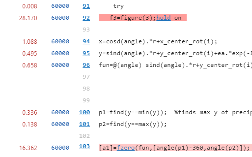
Identifying Optimisations
Once profiling results have been interpreted, the next step is to determine whether there are obvious optimisation opportunities in the components identified as most expensive.
Many of the easiest performance improvements come from eliminating redundant work. This can take several forms. In some cases the issue will be immediately obvious to the code’s author, such as expensive logging, validation, or diagnostics performed on every iteration that could be removed entirely or reduced in frequency. In other cases, profiling highlights expensive calculations, object creation, or other intensive operations that are repeated unnecessarily inside loops and could instead be performed once and reused.
More subtle forms of redundancy are often hidden behind incorrect library usage. For example, passing an inappropriate data type to a library function, such as a Python list to a NumPy function, may trigger an implicit and expensive conversion on every call.
These issues are frequently logical errors rather than complex performance problems, and they can occur within a few lines of code or across several layers of abstraction. Profiling helps focus attention so that these inefficiencies become visible.
Other quick optimisations require more experience to recognise. A common example is using a linear search over a collection such as an array to test for membership. While this approach is intuitive, using a set data structure is often far more appropriate and can be orders of magnitude faster for large inputs.
It is difficult to provide a comprehensive checklist for identifying all possible optimisations. If the most expensive components appear reasonable and no obvious issues stand out, it may be that the code is already performing as well as expected. If doubts remain, there are several practical next steps:
- Look for relevant patterns in the SIG-RPC optimisation database and external resources list, which are regularly updated with new examples.
- Ask a large language model to review a small, self-contained code snippet for performance issues. Providing additional context such as data types and expected input sizes will significantly improve the quality of feedback. Though be aware that LLMs often provide incorrect advice, so you should always verify whether the suggestions actually improve performance and give correct results.
- Request a review from a local Research Software Engineering (RSE) or Research IT team. With profiling results available, experienced developers can often identify potential issues quickly or help investigate less obvious ones.
After applying any optimisation, always re-profile the code and carry out your normal validation. It is important to make sure your optimised code still produces valid results as optimisation changes can introduce subtle correctness issues. A formal test suite is ideal for catching such errors. You may also find at this stage, upon re-profiling, that removing one bottleneck has exposed smaller secondary ones which could be worth optimising too.
A clean profiling report provides additional confidence that your code meets a higher standard of quality, both for running experiments reliably and for publishing reproducible research software. With more experience reviewing your code’s performance, you will find it easier to spot similar issues and potentially even catch them whilst writing code.
Case Studies
We are steadily building a collection of research software profiling case studies. The first published example describes how profiling and optimisation uncovered a tenfold speedup in code that had existed in the codebase for seven years without performance issues being recognised (read the case study).
If you have had success profiling and optimising your own research software, we would welcome a case study written from your perspective. The more examples we can share, the more clearly we can demonstrate the impact that profiling can have on research code.
If you are interested in contributing, you can get in touch to discuss your experience with us, or submit an issue or a pull request directly.
Key Points
The key information to take away from this article is:
- Profiling collects detailed performance metrics and highlights where optimisation will have the greatest impact.
- Focus optimisation on code that accounts for a significant portion of runtime.
- Hot-path profilers come in various types, but most are suitable for standard CPU code. GPU or distributed workloads may require specialised tools.
- Profile code once it is functionally complete and ready for release.
- Use a representative workflow or input, ideally one that runs for several minutes.
- Profiling results are typically visualised as flame or icicle graphs, tables showing the most expensive functions/lines, or inline annotations of the source code.
- When a hotspot is identified, examine it for obvious redundancy or inefficiency. Seek guidance from a Research Software Engineer if unsure.
- After making changes, profile again, as new bottlenecks may appear.
Now that you’ve read through the introductory materials, you should visit our profilers database to find a suitable profiler for your code.